1. Drawing statistical conclusions
Chapter 1 of the Statistical Sleuth
Drawing statistical conclusions
- the two-sample problem
- measure of uncertainty - based on probability model
- when based on chance mechanism (coin flips), measures of uncertainty are formally justified
- often instead invented as conceptual frameworks for drawing statistical conclusions
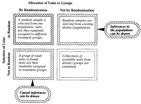
- key question: was chance mechanism used, for sample selection, group allocation, ?
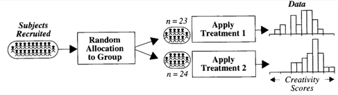
Ex: Creativity and writing - experimental
Two populations, randomly selected to receive treatment.
- Two-sample t-test: two-sided p-value.
- Estimated difference between the two scores 4.1
- 95% confidence interval between 1.3 and 7.0
- strong causal relationship (even though group was not randomized)
Ex: Sex discrimination in employment - observational
Are men paid more than women at a bank
- Starting salary for men $580-$1080 more, 95% confidence interval
- One-sided p-value < .00001 from two-sample t-test
- Difference between one-sided and two-sided p-value?
Inference
Both depending on study design, can be justified by proper use of random mechanisms
Terms
- inference: conclusion that patterns in the data are present in some broader framework
- statistical inference: inference justified by a probability model linking data to a broader context
Kinds
- causal inference
- sometimes, causal is not the goal. for example, knowing that Asian men react different to a medication is important, even if it's because of their diet, not because of their “being Asian”
- theory can help establish causation even without randomization
- inference to populations
- can only be done with random selection
Probability model for randomized experiments (p-values)
Additive treatment effect model
Subject would receive a different creativity score Y* after treatment, ``Y* = Y + delta`` (``delta``=treatment effect, parameter, unknown constant)
Question: Is there a treatment effect → Does the parameter d have a non-zero value?
- Null-hypothesis: ``delta = 0``
- Alternative hypothesis: ``delta != 0``
- Statistic: Numerical quantity calculated from data.
- Test statistic: Statistic used to measure plausibility of an alternative hypothesis relative to a null-hypothesis. d = 0, test-hypothesis = avg(``bar(Y_2)``) - avg(``bar(Y_1)``). If null-hypothesis is true, difference should be small.
OK, so we now that avg(``bar(Y_2)``) - avg(``bar(Y_1)``) = 4.1. Is this a lot? If the null-hypothesis is true, ``delta = 0``, so we could randomize the distribution into two groups in any way we wanted. Theoretically, we could calculate avg(``bar(Y_1)``) and avg(``bar(Y_2)``) for all possible versions of ``bar(Y_1)`` and ``bar(Y_2)``. Let's do that for a 1000 groups. Histogram:
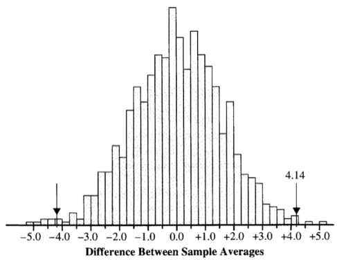
We see that the difference in most cases is between +3 and -3, only four of the 1000 randomizations produced results as large as 4.14, ie. it's an unusually uneven randomization outcome, if the null-hypothesis is correct.
P-values
Observed p-value: In a randomized experiment, the p-value is the probability that randomization alone leads to a test statistic as extreme or more extreme than the one observed.
In this case, 4/1000 observations produced a result as or more extreme, leading to a p-value of 0.004. This is a one-sided p-value for the alternative-hypothesis d > 0. Statistics smaller than -4.1 may provide equally strong evidence against the null-hypothesis, favoring the alternative hypothesis that ``delta < 0``. If those (7) are included, result is a two-sided p-value of 11/1000 = 0.011, appropriate for the two-sided alternative hypothesis that ``d != 0``.
Estimating p-value
Three ways
- calculate all possibilities → observed p-value. Often difficult (millions of possibilities)
- estimate p-values → simulate large number of randomizations (what we just did above) is this connected to Bayesian statistics?
- most common: approximate randomization distribution with a mathematical curve, based on certain assumptions about the distribution of the measurement and the form of the test statistic. so this is why it's so important to check for skewness, kurtosis etc... Does this become less important, if one uses the estimation approach above?
Measuring uncertainty in observational studies
Without randomization we have to approach inference differently. Two approaches.
Non-random sample
Connect distribution of test-statistics to a chance mechanism for sample selection
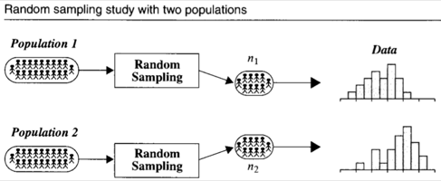
Let's assume we draw a random sample from population 1, ``n_1``, and another random sample from population 2, ``n_2``. The samples are drawn independently. How do these populations differ? Difference between their means, u1 and u2, these become the single parameter for answering questions of interest. Inferences and uncertainty measures based on difference ``bar(Y_2) - bar(Y_1)``, between sample averages, which estimates the difference in population means.
Sampling distribution for ``bar(Y_2) - bar(Y_1)``, represented by histogram of all values for the statistic from all possible samples that can be drawn from the two populations. P-value for testing a hypothesis and the confidence intervals estimating the parameter follow from an understanding of the sampling distribution.
not very clear, more info in chapter 2 apparently
Not a sample (data for every member of the population)
We're not interested in the salaries of people who were not hired, and gender cannot be seen as randomly assigned, thus random sampling and randomized experiment models do not apply. Need to use fictitious chance model.
One possible model: employer assigned starting salaries at random. Q: Is observed difference random?
Permutation distribution of test statistic
Permutation distribution: Collection of differences in averages from all possible assignments of starting salaries to individuals
This is similar to what we did above with p-value, but less certain because of the lack of randomization.
It's extremely improbable that the difference between ``bar(Y_2)`` and ``bar(Y_1)`` would be as high as $820 (p < 0.00001).
What do we know? That the employer did not select starting salaries at random.
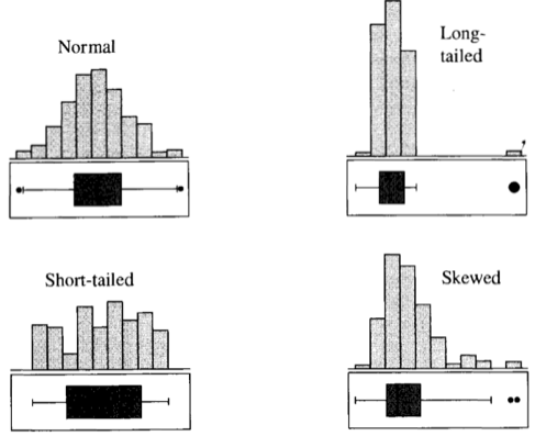
Kinds of graphs
Nice collection of box-plots and histograms, gives an intuitive sense of the distribution and some vocabulary (long-tailed, short-tailed etc).
Vocabulary
- Parameter: unknown numerical value describing feature of a probability model (Greek letters)
- Statistic: quantity that can be calculated from observed data (Roman letters)
- Estimate: statistic used to guess the value of a parameter (Greek letter with ^ hat)
- estimate can be calculated, but parameter remains unknown
- Mean: average of a population (``mu``)
- Average: average of a sample (statistic) (``bar(Y)``)
- Experimental units: things to which treatments are applied
- Two-treatment randomized experiment: all available units have the same chance of being placed in group 1
- Frame: Numbered list of all units of a population (for random sample)
- Systematic random sampling: Choose random beginning number, and then choose every nth unit in a frame
- Random cluster sampling: Sort units into n blocks of size(population)/n units, and choose one of the units randomly
- Variable probability sampling: For example, sampling lakes of different sizes, give large lakes a higher probability of being selected
Standard deviation SD of a set of numbers ``Y_1``…``Y_n``:
``sqrt ( ( sum_(i=1)^n (Y_i - bar(Y) )^2) // (n - 1)``
Population SD (``sigma``), sample SD (s). Measure of spread as distance between a single number, and the set's average.

